Recall Hypothesis Test

A statistical J. Brownlee - Machine Learning Mastery makes an assumption about the outcome, called the null hypothesis.

For example, the null hypothesis for the Pearson’s correlation test is that there is no relationship between two variables. The null hypothesis for the Student’s t test is that there is no difference between the means of two populations.

The test is often interpreted using a P-value, which is the probability of observing the result given that the null hypothesis is true, not the reverse, as is often the case with misinterpretations.

P-value ( $p$ ):
Probability of obtaining a result equal to or more extreme than was observed in the data.
Link to original

In interpreting the $p$ -value of a significance test, you must specify a significance level, $α$ . A common value for the Significance Level is 5% written as 0.05.

The $p$ -value is interested in the context of the chosen Significance Level. A result of a significance test is claimed to be “statistically significant” if the $p$ -value is less than the Significance Level. This means that the null hypothesis (that there is no result) is rejected.

$p \leq α$ : reject H0, different distribution.
$p > α$ : fail to reject H0, same distribution.

Where:

Significance Level ( $α$ ).
Boundary for specifying a statistically significant finding when interpreting the P-value.
Link to original

We can see that the $p$ -value is just a probability and that in actuality the result may be different. The test could be wrong. Given the $p$ -value, we could make an error in our interpretation.

There are two types of errors; they are:

In this context, we can think of the Significance Level as the probability of rejecting the null hypothesis if it were true. That is the probability of making a Type I Error or a false positive.

Statistical Power

Statistical power, or the power of a J. Brownlee - Machine Learning Mastery is the probability that the test correctly rejects the null hypothesis.

That is, the probability of a true positive result. It is only useful when the null hypothesis is rejected.

… statistical power is the probability that a test will correctly reject a false null hypothesis. Statistical power has relevance only when the null is false. [1]

The higher the statistical power for a given experiment, the lower the probability of making a Type II (false negative) error. That is the higher the probability of detecting an effect when there is an effect. In fact, the power is precisely the inverse of the probability of a Type II error.

$Power = 1 - Type II Error$

$P (True Positive) = 1 - P (False Negative)$

More intuitively, the statistical power can be thought of as the probability of accepting an alternative hypothesis, when the alternative hypothesis is true.

When interpreting statistical power, we seek experiential setups that have high statistical power.

Low Statistical Power: Large risk of committing Type II errors, e.g. a false negative.
High Statistical Power: Small risk of committing Type II errors.

Experimental results with too low statistical power will lead to invalid conclusions about the meaning of the results. Therefore a minimum level of statistical power must be sought.

It is common to design experiments with a statistical power of 80% or better, e.g. 0.80. This means a 20% probability of encountering a Type II area. This different to the 5% likelihood of encountering a Type I error for the standard value for the significance level.

Power Analysis

Statistical power is one piece in a puzzle that has four related parts; they are:

Effect Size. The quantified magnitude of a result present in the population. Effect size is calculated using a specific statistical measure, such as Pearson’s correlation coefficient for the relationship between variables or Cohen’s d for the difference between groups.
Sample Size. The number of observations in the sample.
Significance. The significance level used in the statistical test, e.g. alpha. Often set to 5% or 0.05.
Statistical Power. The probability of accepting the alternative hypothesis if it is true.

All four variables are related. For example, a larger sample size can make an effect easier to detect, and the statistical power can be increased in a test by increasing the significance level.

A power analysis involves estimating one of these four parameters given values for three other parameters. This is a powerful tool in both the design and in the analysis of experiments that we wish to interpret using statistical hypothesis tests.

For example, the statistical power can be estimated given an effect size, sample size and significance level. Alternately, the sample size can be estimated given different desired levels of significance.

Power analysis answers questions like “how much statistical power does my study have?” and “how big a sample size do I need?” [2]

Perhaps the most common use of a power analysis is in the estimation of the minimum sample size required for an experiment.

Power analyses are normally run before a study is conducted. A prospective or a priori power analysis can be used to estimate any one of the four power parameters but is most often used to estimate required sample sizes. [3]

As a practitioner, we can start with sensible defaults for some parameters, such as a significance level of 0.05 and a power level of 0.80. We can then estimate a desirable minimum effect size, specific to the experiment being performed. A power analysis can then be used to estimate the minimum sample size required.

In addition, multiple power analyses can be performed to provide a curve of one parameter against another, such as the change in the size of an effect in an experiment given changes to the sample size. More elaborate plots can be created varying three of the parameters. This is a useful tool for experimental design.

Student’s T Test Power Analysis

We can make the idea of statistical power and power analysis concrete with a worked example.

In this section, we will look at the Student’s t test, which is a statistical J. Brownlee - Machine Learning Mastery for comparing the means from two samples of Gaussian variables. The assumption, or null hypothesis, of the test is that the sample populations have the same mean, e.g. that there is no difference between the samples or that the samples are drawn from the same underlying population.

The test will calculate a $p$ -value that can be interpreted as to whether the samples are the same (fail to reject the null hypothesis), or there is a statistically significant difference between the samples (reject the null hypothesis). A common significance level for interpreting the $p$ -value is 5% or 0.05.

Significance level ( $α$ ): 5% or 0.05.

The size of the effect of comparing two groups can be quantified with an effect size measure. A common measure for comparing the difference in the mean from two groups is the Cohen’s d measure. It calculates a standard score that describes the difference in terms of the number of standard deviations that the means are different. A large effect size for Cohen’s d is 0.80 or higher, as is commonly accepted when using the measure.

Effect Size: Cohen’s d of at least 0.80.

We can use the default and assume a minimum statistical power of 80% or 0.8.

Statistical Power: 80% or 0.80.

For a given experiment with these defaults, we may be interested in estimating a suitable sample size. That is, how many observations are required from each sample in order to at least detect an effect of 0.80 with an 80% chance of detecting the effect if it is true (20% of a Type II error) and a 5% chance of detecting an effect if there is no such effect (Type I error).

We can solve this using a power analysis.

The statsmodels library provides the TTestIndPower class for calculating a power analysis for the Student’s t test with independent samples. Of note is the TTestPower class that can perform the same analysis for the paired Student’s t test.

The function solve_power() can be used to calculate one of the four parameters in a power analysis. In our case, we are interested in calculating the sample size. We can use the function by providing the three pieces of information we know (alpha, effect, and power) and setting the size of argument we wish to calculate the answer of (nobs1) to None. This tells the function what to calculate.

A note on sample size: the function has an argument called ratio that is the ratio of the number of samples in one sample to the other. If both samples are expected to have the same number of observations, then the ratio is 1.0. If, for example, the second sample is expected to have half as many observations, then the ratio would be 0.5.

The TTestIndPower instance must be created, then we can call the solve_power() with our arguments to estimate the sample size for the experiment.

# perform power analysis 
analysis = TTestIndPower() 
result = analysis.solve_power(effect, power=power, nobs1=None, ratio=1.0, alpha=alpha)

The complete example is listed below.

# estimate sample size via power analysis 
from statsmodels.stats.power import TTestIndPower 
 
# parameters for power analysis 
effect = 0.8 
alpha = 0.05 
power = 0.8 
 
# perform power analysis 
analysis = TTestIndPower() 
result = analysis.solve_power(effect, power=power, nobs1=None, ratio=1.0, alpha=alpha) 
print('Sample Size: %.3f' % result)

Running the example calculates and prints the estimated number of samples for the experiment as 25. This would be a suggested minimum number of samples required to see an effect of the desired size.

Sample Size: 25.525

We can go one step further and calculate power curves.

Power curves are line plots that show how the change in variables, such as effect size and sample size, impact the power of the statistical test.

The plot_power() function can be used to create power curves. The dependent variable (x-axis) must be specified by name in the dep_var argument. Arrays of values can then be specified for the sample size (nobs), effect size (effect_size), and significance (alpha) parameters. One or multiple curves will then be plotted showing the impact on statistical power.

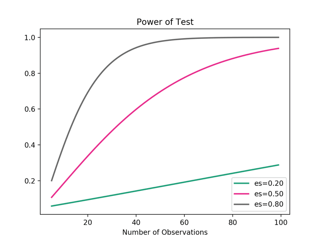
For example, we can assume a significance of 0.05 (the default for the function) and explore the change in sample size between 5 and 100 with low, medium, and high effect sizes.

# calculate power curves from multiple power analyses
analysis = TTestIndPower()
analysis.plot_power(dep_var='nobs', nobs=arange(5, 100), effect_size=array([0.2, 0.5, 0.8]))

The complete example is listed below.

# calculate power curves for varying sample and effect size
from numpy import array
from matplotlib import pyplot
from statsmodels.stats.power import TTestIndPower
# parameters for power analysis
effect_sizes = array([0.2, 0.5, 0.8])
sample_sizes = array(range(5, 100))
# calculate power curves from multiple power analyses
analysis = TTestIndPower()
analysis.plot_power(dep_var='nobs', nobs=sample_sizes, effect_size=effect_sizes)
pyplot.show()

Running the example creates the plot showing the impact on statistical power (y-axis) for three different effect sizes (es) as the sample size (x-axis) is increased.

We can see that if we are interested in a large effect that a point of diminishing returns in terms of statistical power occurs at around 40-to-50 observations.

Power Curves for Student's t Test

Usefully, statsmodels has classes to perform a power analysis with other statistical tests, such as the F-test, Z-test, and the Chi-Squared test.

Extensions

This section lists some ideas for extending the tutorial that you may wish to explore.

Plot the power curves of different standard significance levels against the sample size.
Find an example of a study that reports the statistical power of the experiment.
Prepare examples of a performance analysis for other statistical tests provided by statsmodels.

If you explore any of these extensions, I’d love to know.

Summary

In this tutorial, you discovered the statistical power of a J. Brownlee - Machine Learning Mastery and how to calculate power analyses and power curves as part of experimental design.

Specifically, you learned:

Statistical power is the probability of a J. Brownlee - Machine Learning Mastery of finding an effect if there is an effect to be found.
A power analysis can be used to estimate the minimum sample size required for an experiment, given a desired significance level, effect size, and statistical power.
How to calculate and plot power analysis for the Student’s t test in Python in order to effectively design an experiment.

Do you have any questions?

Ask your questions in the comments below and I will do my best to answer.

References

[1] Page 60, The Essential Guide to Effect Sizes: Statistical Power, Meta-Analysis, and the Interpretation of Research Results, 2010.

[2] Page 56, The Essential Guide to Effect Sizes: Statistical Power, Meta-Analysis, and the Interpretation of Research Results, 2010.

[3] Page 57, The Essential Guide to Effect Sizes: Statistical Power, Meta-Analysis, and the Interpretation of Research Results, 2010.

ML.MD

Explorer

Recall Hypothesis Test

Recall Hypothesis Test

Statistical Power

Power Analysis

Student’s T Test Power Analysis

Extensions

Further Reading

Papers

Books

API

Articles

Summary

References

Graph View

Table of Contents

Backlinks